Definitions of electric power qualities under nonsinusoidal conditions are quite complex and hard to grasp. Annex B of the IEEE Std 1459-2010 shows how to calculate apparent power components in non-sinusoidal conditions. I have written a MATLAB script to illustrate this example. Unfortunately, there were typo errors in the standard, that’s why some of the values are different in my example.
Figure 1 — Instantaneous voltage and current
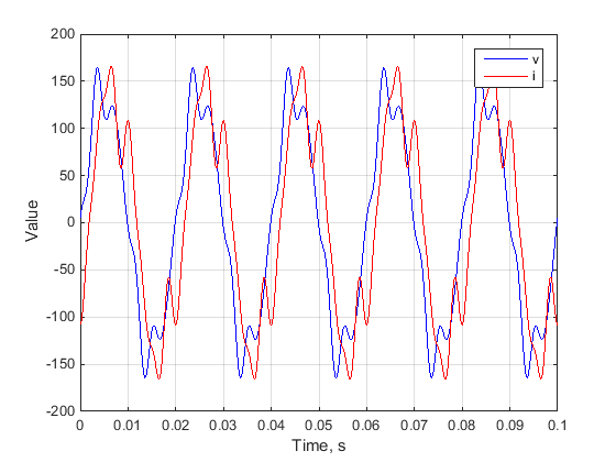
A load is supplied with a nonsinusoidal voltage
\[ v=v_1 + v_3 + v_5 +v_7 = \sqrt{2} \sum_{h=1,3,5,7}V_h \sin(h \omega t-\alpha_h) \]
has a nonsinusoidal current
\[ i=i_1 + i_3 + i_5 +i_7 = \sqrt{2} \sum_{h=1,3,5,7}I_h \sin(h \omega t-\beta_h) \]
(To simplify the explanations, the eventual presence of dc components was ignored.) In this case, the instantaneous power has 16 terms that can be separated in two groups
\[ p=vi=p_{hh}+p_{mn} \]
where
\[ p_{hh}=v_1 i_1 + v_3 i_3 +v_5 i_5 +v_7 i_7 = \sum_{h=1,3,5,7} v_h i_h \]
is the instantaneous power that contains only direct products (i.e., each component is the result of interaction of voltage and current harmonics of the same order).
\[ p_{mn}=v_1 (i_3 +i_5 +i_7) + v_3 (i_1 +i_5 +i_7) +v_5 (i_1 +i_3 +i_7) +v_7 (i_1+i_3+i_7) = \] \[ = \sum_{m=1,3,5,7} v_m \sum_{n =1,3,5,7 \atop n \neq m} i_n \]
is the instantaneous power that contains only cross products (i.e., each component is the result of interaction of voltage and current harmonics of different orders).
The direct products yield
\[ v_h i_h=\sqrt{2} \, V_h \sin (h \omega t - \alpha_h) \sqrt{2} \, I_h \sin (h \omega t - \beta_h) = \] \[ = P_h [1 - \cos(2 h \omega t - 2 \alpha_h)] - Q_h \sin (2 h \omega t - 2 \alpha_h) \]
where
\[ P_h = V_h I_h \cos (\theta_h)\] \[ Q_h =V_h I_h \sin (\theta_h) \]
are the harmonic active and reactive powers of order $ h $, respectively, and $ \theta_h = \beta_h - \alpha_h $ is the phase angle between the phasors $ V_h $ and $ I_h $.
The total active power is
\[ P = \sum_{h=1,3,5,7} P_h =P_1 +P_H \]
where
\[ P_1 = V_1 I_1 \cos(\theta_1) \]
is the fundamental (power-frequency) active power, and
\[ P_H=P_3+P_5+P_7 = \sum_{h \neq 1} P_h \]
is the total harmonic active power.
For each harmonic order, there is an apparent power of order h
\[ S_H=\sqrt{P_h^2 +Q_h^2} \]
The cross-products of the instantaneous powers have expressions as follows:
\[ v_m i_n=\sqrt{2} \, V_m \sin (m \omega t - \alpha_m) \sqrt{2} \, I_n \sin (n \omega t - \beta_n) = \] \[ = D_{mn} \left( \cos[(m-n) \omega t - \alpha_m + \beta_n ] + \cos[(m+n) \omega t - \alpha_m - \beta_n] \right) \]
where
\[ D_{mn}=V_m I_n \]
The total apparent power squared
\[ S^2 = V^2 I^2 =(V_1^2 +V_3^2 +V_5^2 +V_7^2)(I_1^2 +I_3^2 +I_5^2 +I_7^2) \]
may be separated in the same manner as the instantaneous power, in direct and the cross-products:
\[ S^2 = V_1^2 I_1^2 +V_3^2 I_3^2 + V_5^2 I_5^2 + V_7^2 I_7^2 + \] \[ + V_1^2 (I_3^2 +I_5^2 +I_7^2) + I_1^2 (V_3^2 +V_5^2 +V_7^2)+ \] \[ + V_3^2 I_5^2 + V_3^2 I_7^2 + V_5^2 I_3^2 + V_5^2 I_7^2 + V_7^2 I_3^2 + V_7^2 I_5^2 \]
or
\[ S^2 = S_1^2 +S_3^2 +S_5^2 +S_7^2 + \] \[ + D_I^2 +D_V^2 + \] \[ + D_{35}^2+ D_{37}^2 + D_{53}^2 + D_{57}^2 + D_{73}^2 + D_{75}^2 = S_1^2 + S_N^2 \]
where
\[ S_1^2 = P_1^2 + Q_1^2 \]
with $ S_1 $ , $ P_1 $ and $ Q_1 $ are the apparent, active, and reactive fundamental powers, and
\[ S_N^2 = D_I^2 + D_V^2 +S_H^2 \]
where
\[ D_I^2 = V_1^2 (I_3^2 +I_5^2 +I_7^2) \]
is the current distortion power,
\[ D_V^2 = I_1^2 (V_3^2 +V_5^2 +V_7^2) \]
is the voltage distortion power, and
\[ S_H^2 = S_3^2 +S_5^2 +S_7^2 + \] \[ + D_{35}^2+ D_{37}^2 + D_{53}^2 + D_{57}^2 + D_{73}^2 + D_{75}^2 = \] \[ = P_3^2 + P_5^2 + P_7^2 + Q_3^2 + Q_5^2 + Q_7^2 + \] \[ + D_{35}^2+ D_{37}^2 + D_{53}^2 + D_{57}^2 + D_{73}^2 + D_{75}^2 \qquad (1) \]
is the harmonic apparent power
If the load is supplied by a line with a resistance $ r $ the power loss in the line is
\[ \Delta P = r I^2 = \frac{r}{V^2} S^2 = \frac{r}{V^2} (S_1^2 + S_N^2) = \] \[ = \frac{r}{V^2} (P_1^2 +Q_1^2 +D_I^2 +D_V^2 +S_H^2) \qquad (2) \]
It is learned from this expression that every component of $ S $ contributes to the total power loss in the supplying system. This means that not only fundamental active and reactive powers cause losses but also the current and voltage distortion powers as well as the harmonic apparent power cause losses.
The following numerical example is meant to facilitate the understanding of the previous explanations:
The instantaneous voltages and currents are
\[ \begin{array}{c c} v_1=\sqrt{2} \, 100 \sin (\omega t - 0^{\circ} ) & i_1=\sqrt{2} \, 100 \sin (\omega t - 30^{\circ} ) \\ v_3=\sqrt{2} \, 8 \sin (\omega t - 70^{\circ} ) & i_3=\sqrt{2} \, 20 \sin (3 \omega t - 165^{\circ} ) \\ v_5=\sqrt{2} \, 5 \sin (\omega t + 140^{\circ} ) & i_5=\sqrt{2} \, 15 \sin (5 \omega t + 233^{\circ} ) \\ v_7=\sqrt{2} \, 7 \sin (\omega t + 20^{\circ} ) & i_7 =\sqrt{2} \, 10 \sin (7 \omega t + 288^{\circ} ) \\ \end{array} \]
The calculated active powers are summarized in Table 1.
Table 1 — Active powers
\[ \begin{array}{|c|c|c|c|c|c|} \hline P_1 (W) & P_3 (W) & P_5 (W) & P_7 (W) & P (W) & P_H (W) \\ \hline 8660.25 & -13.94 & -11.78 & -1.74 & 8632.79 & -27.47 \\ \hline \end{array} \]
The total harmonic active power $ P_H =P –27.47 W < 0 $ is supplied by the load and injected into the power system. This condition is typical for dominant nonlinear loads. The bulk of the active power is supplied to the load by the fundamental component $ P_1 = 8660.25 W$ .
The four reactive powers are given in Table 2.
Table 2 — Reactive powers
\[ \begin{array}{|c|c|c|c|} \hline Q_1 (var) & Q_3 (var) & Q_5 (var) & Q_7 (var) \\ \hline 5000.00 & 159.39 & -224.69 & 49.97 \\ \hline \end{array} \]
Of interest is the fact that $ Q_5 < 0$ , whereas other reactive powers are positive. If one incorrectly defines a total reactive power as the sum of the four reactive powers (in accordance with C. Budeanu’s definition):
\[ Q_B = Q_1 +Q_3 +Q_5 +Q_7 = 4984.67 \, var \]
and assumes that the supplying line has a resistance $ r= 1.0 \, \Omega $ and the load is supplied with an rms voltage $ V=240 V $, the power loss due to $ Q_B $ in line is
\[ \Delta P_B = \frac{r}{V^2}Q_B^2= \frac{1}{240^2}4984.67^2 = 431.37 \, W \]
According to the previous analysis, [see Equation (1) and Equation (2)], the correct way to find the corresponding power loss due to $ Q_1 $ , $ Q_3 $ , $ Q_4 $ , $ Q_7 $ is
\[ \Delta P = \frac{r}{V^2}(Q_1^2 +Q_3^2 +Q_5^2 +Q_7^2)= 435.39 \, W > P_B \]
The reactive power $ Q_5 $ , despite its negative value, contributes to the line losses in the same way as the positive reactive powers. The fact that harmonic reactive powers of different orders oscillate with different frequencies reinforces the conclusion that the reactive powers should not be added arithmetically (as recommended by Budeanu).
The cross-products that produce the distortion powers $ D_I $ and $ D_V $ are given in Table 3.
Table 3 — Distortion powers and their components
\[ \begin{array}{|c|c|c|c|} \hline D_{13} (var) & D_{15} (var) & D_{17} (var) & D_{I} (var) \\ \hline 2000.00 & 1500.00 & 1000.00 & 2692.58 \\ \hline D_{31} (var) & D_{51} (var) & D_{71} (var) & D_{V} (var) \\ \hline 800.00 & 1500.00 & 500.00 & 1772.00 \\ \hline \end{array} \]
Finally the remaining cross-products that belong to the harmonic apparent power are presented in Table 4.
Table 4 — Distortion harmonic powers
\[ \begin{array}{|c|c|c|c|c|c|} \hline D_{35} (var) & D_{37} (var) & D_{53} (var) & D_{57} (var) & D_{73} (var) & D_{75} (var) \\ \hline 120.00 & 80.00 & 300.00 & 150.00 & 100.00 & 75.00 \\ \hline \end{array} \]
The studied system has the rms voltage and current: $ V= 101.56 \, V $ and $ I= 103.56 \, A $ with the total harmonic distortions $ THD_V = 0.177 $ and $ THD_I = 0.269 $
The apparent power and its components are represented in the following tree:
Figure 2 — Apparent power and its components tree
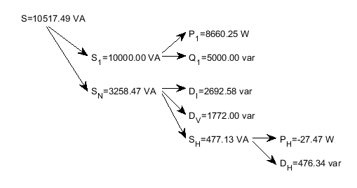
The fundamental power factor (displacement power factor) is $ PF_1 = P_1 / S_1 =0.866 $, and the power factor is $ PF= P/S=0.821 $ . The dominant power components are $ P_1 $ and $ Q_1 $ . Due to relatively large distortion, $ S_N $ is found to be a significant portion of $ S $, and the current distortion power $ D_I $ is the dominant component of $ S_N $ .
Here is the MATLAB script that illustrates the previous material.
1 2 3 4 5 6 7 8 9 10 11 12 13 14 15 16 17 18 19 20 21 22 23 24 25 26 27 28 29 30 31 32 33 34 35 36 37 38 39 40 41 42 43 44 45 46 47 48 49 50 51 52 53 54 55 56 57 58 59 60 61 62 63 64 65 66 67 68 69 70 71 72 73 74 75 76 77 78 79 80 81 82 83 84 85 86 87 88 89 90 91 92 93 94 95 96 97 98 99 100 101 102 103 104 105 106 107 108 109 110 111 112 113 114 115 116 117 118 119 120 121 122 123 124 125 126 127 128 129 130 131 132 133 134 135 136 137 138 139 140 141 142 143 144 145 146 147 148 | |