Umax=1;% Set maximum voltage, for which max ADC code is reachedbits=16;% ADC resolution U=double(uencode(U,bits,Umax,'signed'))/(2^(bits-1))*(Umax);
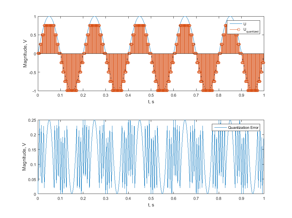
ADC quantization demo
12345678910111213141516
t=0:1/500:1-1/500;U=sin(2*pi*5.00*t);Umax=1;% Set maximum voltage, for which max ADC code is reachedbits=3;% ADC resolution Uq=double(uencode(U,bits,Umax,'signed'))/(2^(bits-1))*(Umax);figure;subplot211plot(t,U),holdon,stem(t,Uq);xlabel('t, s'),ylabel('Magnitude, V');legend('U','U_{quantized}');subplot212plot(t,U-Uq);legend('Quantization Error');xlabel('t, s'),ylabel('Magnitude, V');
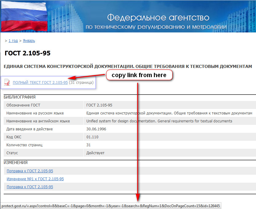
Unfortunately the Russian database of the national standards (GOSTs) does not enable to get files as .pdf , but only as separate images (which are even not directly available).
So we can’t even download the texts, it’s a pity. I’ve made a simple Python script to address this problem, because it’s far better to read and explore a printed copy.
Script uses some libraries, you can install them by running pip install img2pdf pypdf2 requests
It was tested in Python 2.7.
Usage:
Find the standard you want to download from site protect.gost.ru
Get the link, in the example it is http://protect.gost.ru/v.aspx?control=8&baseC=-1&page=0&month=-1&year=-1&search=&RegNum=1&DocOnPageCount=15&id=126445
Replace the link in the script
Run the script python gostdl.py
In the same folder you will get separate pages of document in .pdf and .jpg format as well as merged document in document.pdf
Python 2.7 script ‘gostdl.py’ to download Gost from protect.gost.ru as a pdf file
After the motherboard replacement I’ve got a blue screen of death (BSOD). This can happen after hard disk replacement also.
I’ve used the recipe from here
to recover from this failure.
DJVU is a very good, although not very portable format for books and documents.
PDF is less efficient in compression, but is far more popular and portable. You can easily find
a free PDF reader for any system, for example for iPhone or iPad, but opening and reading DJVU is harder.
But you can always quiclky export DJVU to PDF and then use your favourite PDF reader program. On the iPad I use GoodReader and FoxitReader.
Here are the instructions:
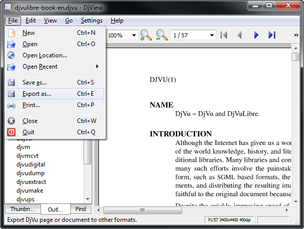
1 - Install DJVULibre. It is available for Windows, Linux and MacOS.
2 - Use File -> Export As…
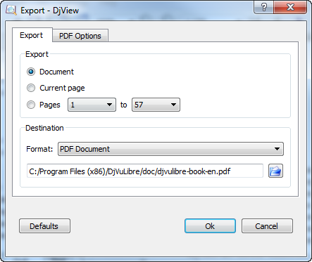
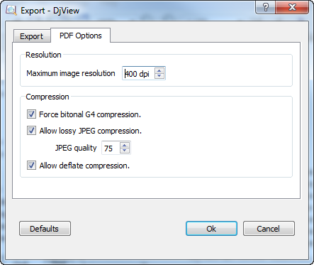
3 - Choose export settings
4 - Choose compression settings
5 - You can also convert books from the command line (good for batch procesing)
command line DJVU to PDF conversion (B & W mode good for most of the books)
Definitions of electric power qualities under nonsinusoidal conditions are quite complex and hard to grasp.
Annex B of the IEEE Std 1459-2010 shows how to calculate apparent power components in non-sinusoidal conditions. I have written a MATLAB script to illustrate this example. Unfortunately, there were typo errors in the standard, that’s why some of the values are different in my example.
(To simplify the explanations, the eventual presence of dc components was ignored.)
In this case, the instantaneous power has 16 terms that can be separated in two groups
is the instantaneous power that contains only direct products (i.e., each component is the result of interaction of voltage and current harmonics of the same order).
is the instantaneous power that contains only cross products (i.e., each component is the result of interaction of voltage and current harmonics of different orders).
The direct products yield
\[
v_h i_h=\sqrt{2} \, V_h \sin (h \omega t - \alpha_h) \sqrt{2} \, I_h \sin (h \omega t - \beta_h) =
\]
\[
= P_h [1 - \cos(2 h \omega t - 2 \alpha_h)] - Q_h \sin (2 h \omega t - 2 \alpha_h)
\]
are the harmonic active and reactive powers of order $ h $, respectively, and
$ \theta_h = \beta_h - \alpha_h $ is the phase angle
between the phasors $ V_h $ and $ I_h $.
The total active power is
\[
P = \sum_{h=1,3,5,7} P_h =P_1 +P_H
\]
where
\[
P_1 = V_1 I_1 \cos(\theta_1)
\]
is the fundamental (power-frequency) active power, and
\[
P_H=P_3+P_5+P_7 = \sum_{h \neq 1} P_h
\]
is the total harmonic active power.
For each harmonic order, there is an apparent power of order h
\[
S_H=\sqrt{P_h^2 +Q_h^2}
\]
The cross-products of the instantaneous powers have expressions as follows:
It is learned from this expression that every component of $ S $ contributes to the total power loss in the supplying system. This means that not only fundamental active and reactive powers cause losses but also the current and voltage distortion powers as well as the harmonic apparent power cause losses.
The following numerical example is meant to facilitate the understanding of the previous explanations:
The total harmonic active power $ P_H =P –27.47 W < 0 $ is supplied by the load and injected into the power system. This condition is typical for dominant nonlinear loads. The bulk of the active power is supplied to the load by the fundamental component $ P_1 = 8660.25 W$ .
Of interest is the fact that $ Q_5 < 0$ , whereas other reactive powers are positive. If one incorrectly defines a total reactive power as the sum of the four reactive powers (in accordance with C. Budeanu’s definition):
\[
Q_B = Q_1 +Q_3 +Q_5 +Q_7 = 4984.67 \, var
\]
and assumes that the supplying line has a resistance $ r= 1.0 \, \Omega $ and the load is supplied with an rms voltage $ V=240 V $, the power loss due to $ Q_B $ in line is
According to the previous analysis, [see Equation (1) and Equation (2)], the correct way to find the corresponding power loss due to $ Q_1 $ , $ Q_3 $ , $ Q_4 $ , $ Q_7 $ is
\[
\Delta P = \frac{r}{V^2}(Q_1^2 +Q_3^2 +Q_5^2 +Q_7^2)= 435.39 \, W > P_B
\]
The reactive power $ Q_5 $ , despite its negative value, contributes to the line losses in the same way as the positive reactive powers. The fact that harmonic reactive powers of different orders oscillate with different frequencies reinforces the conclusion that the reactive powers should not be added arithmetically (as recommended by Budeanu).
The cross-products that produce the distortion powers $ D_I $ and $ D_V $ are given in Table 3.
The studied system has the rms voltage and current:
$ V= 101.56 \, V $ and $ I= 103.56 \, A $ with the total harmonic distortions
$ THD_V = 0.177 $ and $ THD_I = 0.269 $
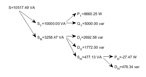
The apparent power and its components are represented in the following tree:
Figure 2 — Apparent power and its components tree
The fundamental power factor (displacement power factor) is $ PF_1 = P_1 / S_1 =0.866 $, and the power factor is $ PF= P/S=0.821 $ . The dominant power components are $ P_1 $ and $ Q_1 $ . Due to relatively large distortion, $ S_N $ is found to be a significant portion of $ S $, and the current distortion power $ D_I $ is the dominant component of $ S_N $ .
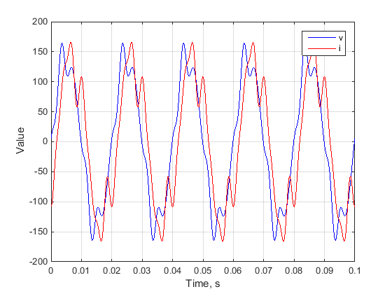
Here is the MATLAB script that illustrates the previous material.
clearall;clc;f_d=12800;% sampling frequencyF=50;% Mains frequencyt=0:1/f_d:1-1/f_d;% timew=2*pi*F;% circular frequency% Magnitudes of the fundamental component and harmonicsV1=100;V3=8;V5=15;V7=5;I1=100;I3=20;I5=15;I7=10;% Angles of the fundamental component and harmonicsphiv1=deg2rad(0);phiv3=deg2rad(-70);phiv5=deg2rad(140);phiv7=deg2rad(20);phii1=deg2rad(-30);phii3=deg2rad(-165);phii5=deg2rad(233);phii7=deg2rad(288);% instantaneous valuesv1=sqrt(2)*V1*sin(w*t+phiv1);v3=sqrt(2)*V3*sin(3*w*t+phiv3);v5=sqrt(2)*V5*sin(5*w*t+phiv5);v7=sqrt(2)*V7*sin(7*w*t+phiv7);v=v1+v3+v5+v7;i1=sqrt(2)*I1*sin(w*t+phii1);i3=sqrt(2)*I3*sin(3*w*t+phii3);i5=sqrt(2)*I5*sin(5*w*t+phii5);i7=sqrt(2)*I7*sin(7*w*t+phii7);i=i1+i3+i5+i7;% theoretical RMS, calculated from magnitudesV=sqrt(V1^2+V3^2+V5^2+V7^2);I=sqrt(I1^2+I3^2+I5^2+I7^2);% actual RMS, calculated from signalsV_RMS=sqrt(1/length(t)*sum(v.*v));I_RMS=sqrt(1/length(t)*sum(i.*i));P1=1/length(t)*sum(v1.*i1);% Fundamental active power (W) 3.1.2.4P3=1/length(t)*sum(v3.*i3);P5=1/length(t)*sum(v5.*i5);P7=1/length(t)*sum(v7.*i7);Q1=V1*I1*sin(phiv1-phii1);% Fundamental reactive power (var) 3.1.2.6Q3=V3*I3*sin(phiv3-phii3);Q5=V5*I5*sin(phiv5-phii5);Q7=V7*I7*sin(phiv7-phii7);% Cross distortion powersD13=V1*I3;D15=V1*I5;D17=V1*I7;D31=V3*I1;D51=V5*I1;D71=V7*I1;%D35=V3*I5;D37=V3*I7;D53=V5*I3;D57=V5*I7;D73=V7*I3;D75=V7*I5;%P=P1+P3+P5+P7;PH=P-P1;% Harmonic active power (nonfundamental active power) (W) 3.1.2.5QB=Q1+Q3+Q5+Q7;% Reactive power (Budenau definition) (not used in 1459)THDV=sqrt((V/V1)^2-1);% Total voltage harmonic distortion (THDV) 3.1.2.1THDI=sqrt((I/I1)^2-1);% Total current harmonic distortion (THDI) 3.1.2.1S=V*I;% Apparent power (VA) 3.1.2.7S1=V1*I1;% Fundamental apparent power (VA) 3.1.2.8SN=sqrt(S^2-S1^2);% Nonfundamental apparent power (VA) 3.1.2.9DI=S1*THDI;% Current distortion power (var) 3.1.2.10DV=S1*THDV;% Voltage distortion power (var) 3.1.2.11SH=S1*THDI*THDV;% Harmonic apparent power (VA) 3.1.2.12DH=sqrt(SH^2-PH^2);% Harmonic distortion power (var)PF1=P1/S1;% Fundamental power factor 3.1.2.15PF=P/S;% Power factor 3.1.2.16% draw figuresfigure;plot(t,v,'b');holdon;plot(t,i,'r');grid;xlim([00.1]);xlabel('Time, s');ylabel('Value');legend('v','i');% draw phasor diagramV1_phasor=V1*exp(1i*phiv1);V3_phasor=V3*exp(1i*phiv3);V5_phasor=V5*exp(1i*phiv5);V7_phasor=V7*exp(1i*phiv7);I1_phasor=I1*exp(1i*phii1);I3_phasor=I3*exp(1i*phii3);I5_phasor=I5*exp(1i*phii5);I7_phasor=I7*exp(1i*phii7);figure;compass(V1_phasor,'b');holdon;compass(V3_phasor,'g');compass(V5_phasor,'r');compass(V7_phasor,'k');compass(I1_phasor,'b--');compass(I3_phasor,'g--');compass(I5_phasor,'r--');compass(I7_phasor,'k--');legend('V1','V3','V5','V7','I1','I3','I5','I7');% draw apparent power and its components treefigure;axis([0101]);axisoff;text(0,1,['S='num2str(S,'%6.2f')' VA']);annotation('arrow',[0.20.3],[0.90.8]);annotation('arrow',[0.1950.3],[0.90.68]);text(0.23,0.83,['S_1='num2str(S1,'%6.2f')' VA']);text(0.23,0.69,['S_N='num2str(SN,'%6.2f')' VA']);annotation('arrow',[0.490.55],[0.80.8]);annotation('arrow',[0.490.55],[0.810.88]);text(0.55,0.93,['P_1='num2str(P1,'%6.2f')' W']);text(0.55,0.83,['Q_1='num2str(Q1,'%6.2f')' var']);text(0.55,0.69,['D_I='num2str(DI,'%6.2f')' var']);text(0.55,0.59,['D_V='num2str(DV,'%6.2f')' var']);text(0.55,0.49,['S_H='num2str(SH,'%6.2f')' VA']);text(0.85,0.49,['P_H='num2str(PH,'%6.2f')' W']);text(0.85,0.39,['D_H='num2str(DH,'%6.2f')' var']);annotation('arrow',[0.490.55],[0.690.69]);annotation('arrow',[0.490.55],[0.680.60]);annotation('arrow',[0.490.55],[0.670.52]);annotation('arrow',[0.720.78],[0.520.52]);annotation('arrow',[0.720.78],[0.510.43]);
To evaluate voltage unbalance we can use Symmetrical components method proposed by Charles Fortescue.
Vector of three phase voltages can be expressed as a sum of three vectors (phasors): zero- positive- and negative-sequence.
Here is MATLAB script that produces the desired level of both negative- and -zero voltage unbalance ratio, then sets respective phasor magnitudes.
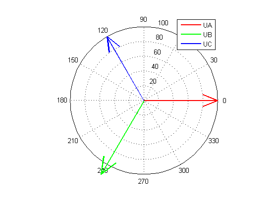
After that we estimate unbalance using Symmetrical components method and draw a phasor diagramm.
clearall;clc;% K2U and K0U calculator% in three phase system we accept that UB lags UA, and UC leads UA% in balanced three phase system all angles are 120 deg=2*pi/3 rad% color coding: UA=red UB=green UC=blueK2U_ref=0.05;% set K2U = 5%% magnitudes of the three phase voltages (rms)mag_UA=100;mag_UB=mag_UA*(1+2*K2U_ref)/(1-K2U_ref);% set magnitude so that K2U=K0U=K2U_refmag_UC=100;% angles of voltagesphi_A=degtorad(0);% absolute angle of UA phasorphi_AB=degtorad(-120);% relative angle between UA phasor and UB phasor% = phi_B-phiA phi_AC=degtorad(120);% relative angle between UA phasor and UC phasor% = phi_C-phiAUA=mag_UA*exp(1i*(phi_A));UB=mag_UB*exp(1i*(phi_A+phi_AB));UC=mag_UC*exp(1i*(phi_A+phi_AC));% calculate symmetrical componentsa=exp(1i*2*pi/3);% complex angle constanta2=a^2;PSP=1/3*(1*UA+a*UB+a2*UC);% Positive sequence phasorNSP=1/3*(1*UA+a2*UB+a*UC);% Negative sequence phasorZSP=1/3*(1*UA+1*UB+1*UC);% Zero sequence phasor% calculate K2U and K0U based on symmetrical componentsK2U=abs(NSP)/abs(PSP)*100% negative sequence ratioK0U=abs(ZSP)/abs(PSP)*100% zero sequence ratioROTATE_UI=angle(UA);% draw phasors relative to UAfigure;h=compass(UA*exp(-1i*ROTATE_UI),'r');holdon;set(h,'LineWidth',2);h=compass(UB*exp(-1i*ROTATE_UI),'g');set(h,'LineWidth',2);h=compass(UC*exp(-1i*ROTATE_UI),'b');set(h,'LineWidth',2);legend('UA','UB','UC');
To generate signal with known level of unbalance $K_{2U}$ we can change magnitude of one of the voltages in the balanced three phase system.
So we set all angles between voltages = 120 deg. Magnitudes of Ua and Uc should be equal (Ua=Uc). Ub should be set as
\[
U_b = U_a \frac{1+2 K_{2U} }{1-K_{2U}}
\]
This equation can be easily derived if we notice that
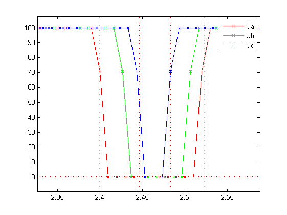
Often we need to draw a vertical or horizontal line across the plot, to mark the boundaries or min/max value of the function. It’s not obvious at the first glance how to do it, becase the X and Y limits can be different, and also we need to handle zoom commands.
I’m now using the solution, based on graph2d.constantline which was found here
Drawing horizontal and vertical lines in MATLAB plot
MATLAB functions that export values into a .CSV file are very slow. It is said, that their inefficiency is rooted in bad implementation of the string concatenation.
It is refered as Schlemiel the Painter’s algorithm.
Nevertheless, sometimes I have to write huge amounts of text data into CSV files. For example I had to generate test signals for power quality measurements algoritms, such as Flicker estimation.
So I had written a MEX function to speed up this task. Write process can also be interrupted by pressing Ctrl-C using this wonderful trick (http://www.caam.rice.edu/~wy1/links/mex_ctrl_c_trick/).
I use Coursera-dl to download lecture videos and materials from Coursera, so I can watch them later after the course is finished.
How to install coursera-dl on Windows machine? It’s easy.
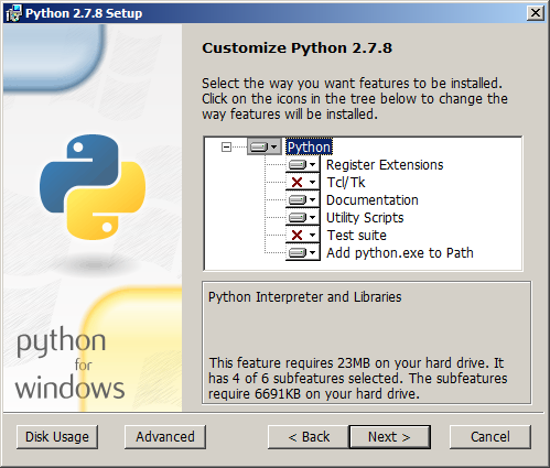
1.First of all you need to download Python 2.7 (don’t download Python 3, it is a different and incompatible version)
from Python download page.
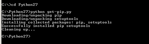
Change directory to your Python installation ( C:\Python27 for my case )
execute python get-pip.py
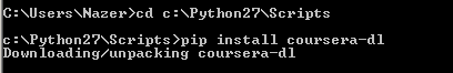
3.Install Coursera-dl script
In the command line change directory to pip (C:\Python27\Scripts for my case)
execute pip install coursera-dl
4.Now you are ready to download materials! For this you need the class name identificator from the browser URL.
Provide your user name and password, directory to download and class name identificator as the parameters into coursera-dl script.
Don’t forget, that you have to accept the honor code of the class before using this script (happens the very first time you go to the class page).
Sample command line to download Coursera materials for current Machine Learning class